分类
二分类-单层感知机-iris数据集
数据分析
(数学原理推断都写在笔记本上了,纸质的,应该没有人需要,我也就不放上来了。)
书上的数据都过于简单了,虽然才刚刚开始学基础,但我还是想是一些比较实用的数据,能带给我一些成就感。这次我使用的是 iris 数据集。这也是我第一次尝试通过数学概念直接写代码,不看书,希望自己能成功。
数据中一共有五列,前四列代表着花萼长度、花萼宽度、花瓣长度、花瓣宽度,我们取前两列作分析。为了方便处理数据,我们将 “Iris-setosa” 定义为1, 将 “Iris-versicolor” 定义为 -1 , 暂时不研究第三类 “Iris-virginica” , 取到第 100 行, 先展示一下数据吧。
因为 numpy 的 loadtxt 功能面对复杂的数据集实在不是很好用,我决定要慢慢地接受使用 pandas 了。目前会慢慢过度。
import numpy as np
import pandas as pd
import matplotlib.pyplot as plt

train = np.array(pd.read_csv('cf-iris.csv').iloc[:100])   # 前 100 行作为训练集
train_x = train[:,0:2]
train_y = np.where(train[:, 4] == 'Iris-setosa', 1, -1)

plt.plot(train_x[train_y == 1, 0], train_x[train_y == 1, 1], 'o')
plt.plot(train_x[train_y == -1, 0], train_x[train_y == -1, 1], 'x')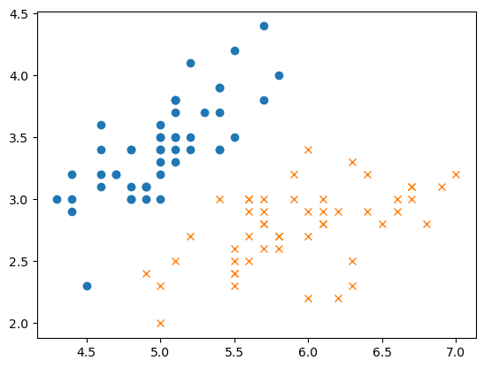
判别函数
我们发现,这个数据是线性可分的,于是尝试用单层感知机进行分类。
\begin{equation} y(x)=\left\{ \begin{aligned} -1 \quad \mathbf{x}\mathbf{\omega} \geq 0\\ 1 \quad \mathbf{x}\mathbf{\omega} < 0\\ \end{aligned} \right . \end{equation}
w = np.random.rand(2)

def f(x):
    return 1 if np.dot(w, x) >= 0 else -1
更新表达式
\begin{equation} \mathbf{\omega}=\left\{ \begin{aligned} \mathbf{\omega}+y^{(i)}x^{(i)} \quad f_\omega(x) \neq y^{(i)}\\ \mathbf{\omega} \quad f_\omega(x) = y^{(i)}\\ \end{aligned} \right . \end{equation}
epoch = 5000 # 重复次数
count = 0
for _ in range(epoch):
    # zip() 返回一个迭代器,将数组 train_x 和 train_y 重新打包成一个多元数组
    for x, y in zip(train_x, train_y):
        if f(x) != y:
            w = w + y*x
            count += 1
            # print('第{}次: w = {}'.format(count, w))
效果展示
对 移项变形得到
绘图展示:
x1 = np.arange(4, 7.5)

plt.plot(train_x[train_y == 1, 0], train_x[train_y == 1, 1], 'o')
plt.plot(train_x[train_y == -1, 0], train_x[train_y == -1, 1], 'x')
plt.plot(x1, -w[0] / w[1] * x1, linestyle = 'dashed')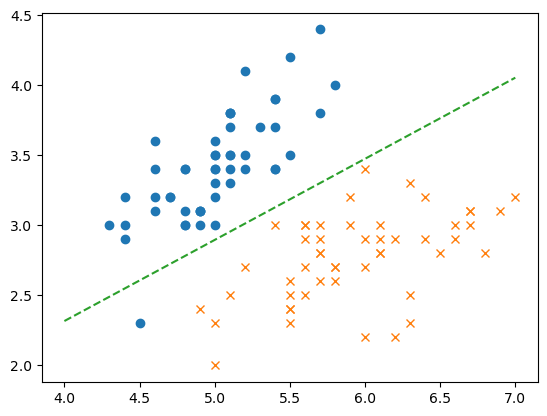
效果还是挺不错的,但是这里踩了一个坑,就是训练次数如果太小的话会导致看不到效果,因为数据前面的内容全都是一个类别的,最好把训练次数调大一点。
分类-逻辑回归
数据准备
逻辑回归中,y 值更适合用 0, 1 表示,首先调整一下。然后对 x 要进行标准化。
train_y = np.where(train_y == -1, 0, train_y)

mu = train_x.mean()
sigma = train_x.std()

# 标准化
def standarize(x):
    return (x - mu) / sigma

train_z = standarize(train_x)

plt.plot(train_z[train_y == 1, 0], train_z[train_y == 1, 1], 'o')
plt.plot(train_z[train_y == -1, 0], train_z[train_y == -1, 1], 'x')

# 增加x0
def to_matrix(x):
    x0 = np.ones([x.shape[0], 1])
    return np.hstack([x0, x])

X = to_matrix(train_z)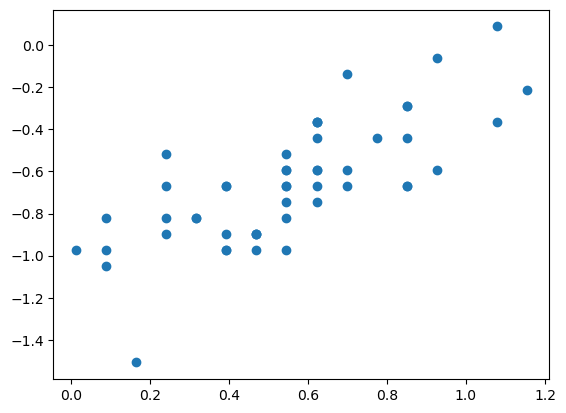
Sigmoid 函数与似然函数
本章的函数比较难推理,建议自己写一遍,以后我应该会录视频专门讲一下机器学习数学基础。
sigmoid 函数:
判别函数:
$y = \left{ \begin{array}{ll}
1, &\theta^T x \geq 0 \
0, &\theta^T x < 0
\end{array} \right. $
似然函数:
整体概率用乘积表示,且此时只有两类情况,所以可以全部用 表示:
参数更新
求导过程有点复杂,我写在笔记本上了,以后有时间应该会以视频或者图片的方式上传。
theta = np.random.rand(3)


# 超级逆天的,花了我整整一天时间,如果不转元素类型为np.float64就会报错
# 猜想:读如数据时使用的是 pandas, 而并非 numpy, 读入的时候就变成了 python 中的 float. 因此和书上不一样
def f(x):
    result = -np.dot(x, theta)
    if not isinstance(result, np.float64):
        return  1 / (1 + np.exp(result.astype(np.float64)))
    else:
        return  1 / (1 + np.exp(result))

# 分类检验
def classify(x):
    return (f(x) >= 0.5).astype(int)


# 学习率
ETA = 1e-3

# 重复次数
epoch = 5000

# 重复学习
for _ in range(epoch):
    theta = theta - ETA * np.dot(f(X) - train_y, X)
结果展示
x0 = np.linspace(-0, 1.5, 100)
plt.plot(train_z[train_y == 1, 0], train_z[train_y == 1, 1], "o")
plt.plot(train_z[train_y == 0, 0], train_z[train_y == 0, 1], "x")

plt.plot(x0, -(theta[0] + theta[1] * x0) / theta[2], linestyle="dashed")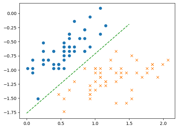
线性不可分的实现
数据准备
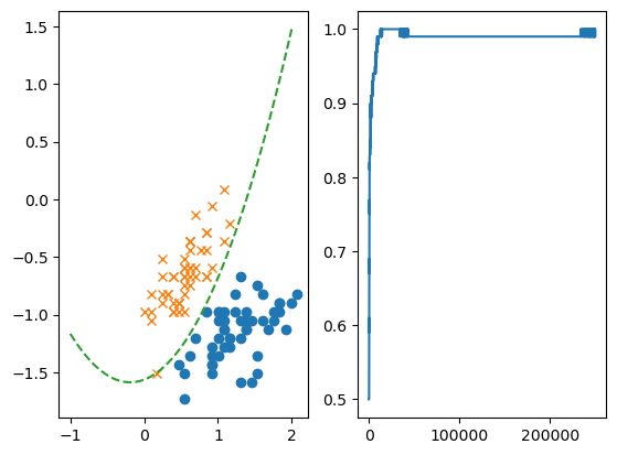
这一次我们使用 50~150 行作为训练数据,并将 Iris-versicolor 设为 1, Iris-virginica 设为 0 ,并用 petal length, petal width 作为分类依据。
这些数据不是很适合线性不可分,还是沿用之前的数据吧,毕竟之前并没有完美的归类。
数据展示:
train = np.array(pd.read_csv('cf-iris.csv').iloc[:100])
train_x = train[:, 0:2]
train_y = np.where(train[:, 4] == 'Iris-versicolor', 1, 0)
train_z = standarize(train_x)

plt.plot(train_z[train_y == 1, 0], train_z[train_y == 1, 1], 'o')
plt.plot(train_z[train_y == 0, 0], train_z[train_y == 0, 1], 'x')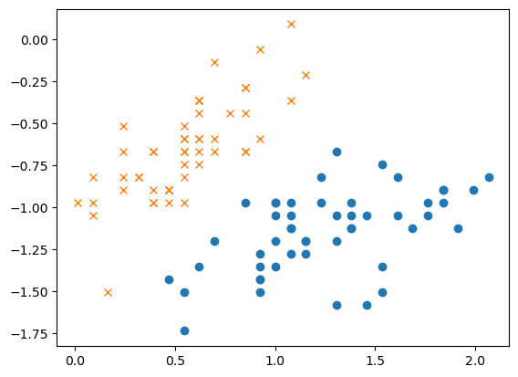
更新 to_matrix 对应向量 theta
我们使用二次函数来拟合决策边界:
def to_matrix(x):
    x0 = np.ones([x.shape[0], 1])
    x3 = x[:, 0, np.newaxis] ** 2 # np.newaxis 用于增加一个额外的维度
    return np.hstack([x0, x, x3]) # 对应 x0(1), x1, x2, x1^2

X = to_matrix(train_z)
重复学习
theta = np.random.rand(4)
ETA = 1e-2
epoch = 2500
# sigmoid 函数不变,就不重复写了

for _ in range(epoch):
    theta = theta - ETA * np.dot(f(X) - train_y, X)
数据展示
x1 = np.linspace(-1, 2, 100)
x2 = -(theta[0] + theta[1]*x1 + theta[3]*x1**2)/theta[2]

plt.plot(train_z[train_y == 1, 0], train_z[train_y == 1, 1], "o")
plt.plot(train_z[train_y == 0, 0], train_z[train_y == 0, 1], "x")
plt.plot(x1, x2, linestyle='dashed')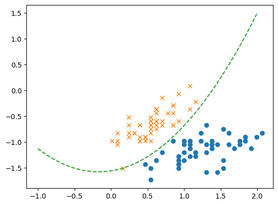
精度曲线 与 随即梯度下降法
# 还是数据的问题,使用不太熟练,只能用笨一点的方法了
def f(x):
    result = -np.dot(x, theta)
    return  1 / (1 + np.exp(np.float64(result)))

theta = np.random.rand(4)

accuracies = []

for _ in range(epoch):
    p = np.random.permutation(X.shape[0])
    for x, y in zip(X[p, :], train_y[p]):
        theta = theta - ETA * (f(x) - y) * x
        result = classify(X) == train_y
        accuracy = len(result[result == True]) / len(result)
        accuracies.append(accuracy)

fig = plt.figure()
ax1 = fig.add_subplot(1, 2, 1)

x1 = np.linspace(-1, 2, 100)
x2 = -(theta[0] + theta[1]*x1 + theta[3]*x1**2)/theta[2]

plt.plot(train_z[train_y == 1, 0], train_z[train_y == 1, 1], "o")
plt.plot(train_z[train_y == 0, 0], train_z[train_y == 0, 1], "x")
plt.plot(x1, x2, linestyle='dashed')

ax2 = fig.add_subplot(1, 2, 2)
x1 = np.arange(len(accuracies))
plt.plot(x1, accuracies)